Kalman Filter For Dummies
A mathematically challenged man's search for scientific wisdom
When I started doing my homework for Optimal Filtering for Signal Processing class, I said to myself :"How hard can it be?". Soon I realized that it was a fatal mistake.
The whole thing was like a nightmare. Nothing made sense. The equations were composed of some ridiculously complex superscripted and subscripted variables combined with transposed matrices and untransposed some other stuff, which are totally unknowable to most of us.
And then, instead of aiming for the homework, I decided first fully concentrating on Kalman Filter itself. This article is the result of my couple of day's work and reflects the slow learning curves of a "mathematically challenged" person.
If you're humble enough to admit that you don't understand this stuff completely, you'll find this material very enlightening.
So, enjoy it!
Kalman Filter
too complicated?
A Quick Insight
As I mentioned earlier, it's nearly impossible to grasp the full meaning of Kalman Filter by starting from definitions and complicated equations (at least for us mere mortals).
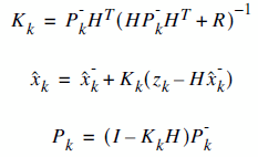
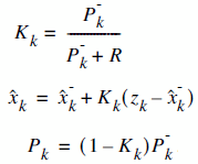
For most cases, the state matrices drop out and we obtain the below equation, which is much easier to start with.

Remember, the k's on the subscript are states. Here we can treat it as discrete time intervals, such as k=1 means 1ms, k=2 means 2ms.
Our purpose is to find  ,
the estimate of the signal x. And we wish to find it for each consequent k's.
Also here,  is the measurement value.
Keep in mind that, we are not perfectly sure of these values. Otherwise, we won't be needing to do all these.
And
  is called "Kalman Gain"
(which is the key point of all these), and
  is the estimate of the signal on the previous state.
The only unknown component in this equation is the  Kalman gain.
Because, we have the measurement values, and we already have the previous estimated signal.
You should calculate this Kalman Gain for each consequent state. This is not easy of course, but we have all the tools to do it.
On the other hand, let's assume  be 0.5,
what do we get? It's a simple averaging! In other words, we should find smarter
 coefficients at each state. The bottom line is :
Kalman filter finds the most optimum averaging factor for each consequent state. Also somehow remembers a little bit about the past states.
Isn't this amazing?
Step-by-Step Guide
Here's a simple step-by-step guide for a quick start to Kalman filtering.
STEP 1 - Build a Model
It's the most important step. First of all, you must be sure that, Kalman filtering conditions fit to your problem.
As we remember the two equations of Kalman Filter is as follows:


It means that each xk (our signal values) may be evaluated by using a linear stochastic equation (the first one). Any xk is a linear combination of its previous value plus a control signal k and a process noise (which may be hard to conceptualize). Remember that, most of the time, there's no control signal uk.
The second equation tells that any measurement value (which we are not sure its accuracy) is a linear combination of the signal value and the measurement noise. They are both considered to be Gaussian.
The process noise and measurement noise are statistically independent.
The entities A, B and H are in general form matrices. But in most of our signal processing problems, we use models such that these entities are just numeric values. Also as an additional ease, while these values may change between states, most of the time, we can assume that they're constant.
If we are pretty sure that our system fits into this model (most of the systems do by the way), the only thing left is to estimate the mean and standard deviation of the noise functions Wk-1 and vk. We know that, in real life, no signal is pure Gaussian, but we may assume it with some approximation.
This is not a big problem, because we'll see that the Kalman Filtering Algorithm tries to converge into correct estimations, even if the Gaussian noise parameters are poorly estimated.
The only thing to keep in mind is : "The better you estimate the noise parameters, the better estimates you get."
STEP 2 - Start the Process
If you succeeded to fit your model into Kalman Filter, then the next step is to determine the necessary parameters and your initial values.
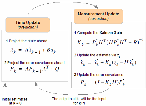
We have two distinct set of equations : Time Update (prediction) and Measurement Update (correction). Both equation sets are applied at each kth state.
| Time Update (prediction) |
Measurement Update (correction) |
 |
 |
We made the modeling in STEP1, so we know the matrices A, B and H. Most probably, they will be numerical constants. And even most probably, they'll be equal to 1.
I suggest you to re-write these equations and see how simplified will these equations become. (if you're lazy enough not to do it, I'll do it for you in the Example below).
The most remaining painful thing is to determine R and Q. R is rather simple to find out, because, in general, we're quite sure about the noise in the environment. But finding out Q is not so obvious. And at this stage, I can't give you a specific method.
To start the process, we need to know the estimate of x0, and P0.
STEP 3 - Iterate
After we gathered all the information we need and started the process, now we can iterate through the estimates. Keep in mind that the previous estimates will be the input for the current state.

Here,  is the prior estimate which in a way, means the rough estimate before the measurement update correction.
And also
  is
the prior error covariance. We use these prior values in our Measurement Update equations.
In Measurement Update equations, we really find  which is the estimate of x at time k (the very thing we wish to find).
Also, we find
  which is necessary for the k+1 (future) estimate,
together with
  .
.
The Kalman Gain ( ) we evaluate
is not needed for the next iteration step, it's a hidden, mysterious and the most important part of this set of equations.
The values we evaluate at Measurement Update stage are also called posterior values. Which also makes sense.
A Simple Example
Now let's try to estimate a scalar random constant, such as a "voltage reading" from a source. So let's assume that it has a constant value of aV (volts), but of course we some noisy readings above and below a volts. And we assume that the standard deviation of the measurement noise is 0.1 V.
Now let's build our model:


As I promised earlier, we reduced the equations to a very simple form.
- Above all, we have a 1 dimensional signal problem, so every entity in our model is a numerical value, not a matrix.
- We have no such control signal uk, and it's out of the game
- As the signal is a constant value, the constant A is just 1, because we already know that the next value will be same as the previous one. We are lucky that we have a constant value in this example, but even if it were any other linear nature, again we could easily assume that the value A will be 1.
- The value H = 1, because we know that the measurement is composed of the state value and some noise. You'll rarely encounter real life cases that H is different from 1.
And finally, let's assume that we have the following measurement values:
| TIME (ms) | 1 | 2 | 3 | 4 | 5 | 6 | 7 | 8 | 9 | 10 |
| VALUE (V) | 0.39 | 0.50 | 0.48 | 0.29 | 0.25 | 0.32 | 0.34 | 0.48 | 0.41 | 0.45 |
OK, we should start from somewhere, such as k=0. We should find or assume some initial state.
Here, we throw out some initial values. Let's assume estimate of X0 = 0,
and P0 = 1. Then why didn't we choose P0 = 0 for example?
It's simple. If we chose that way, this would mean that there's no noise in the environment,
and this assumption would lead all the consequent  to be zero (remaining as the initial state). So we choose P0 something other that zero.
Let's write the Time Update and Measurement Update equations.
| Time Update (prediction) |
Measurement Update (correction) |
 |
 |
Now, let's calculate the  values for each iteration.
| k |  |
 |
 |
Time Update | Measurement Update |  |
 |
|---|---|---|---|---|---|---|---|
| 1 | 0.390 | 0 | 1 |
 = =
 = 0 = 0
 = =
 = 1 = 1
|
 = 1 / (1 0.1) = 1 / (1 0.1)
= 0.909  = 0.909 . (0.390 - 0) = 0.909 . (0.390 - 0)
= 0.35  = (1 - 0.909) . 1 = (1 - 0.909) . 1
= 0.091 |
0.355 | 0.091 |
| 2 | 0.500 | 0.355 | 0.091 |
 = 0.355 = 0.355
 = 0.091 = 0.091
|
 = 0.091 / (0.091 0.1) = 0.091 / (0.091 0.1)
= 0.476  = 0.355 . 0.476 . (0.500 - 0.355) = 0.355 . 0.476 . (0.500 - 0.355)
= 0.424  = (1 - 0.476) . 0.091 = (1 - 0.476) . 0.091
= 0.048 |
0.424 | 0.048 |
| 3 | 0.480 | 0.424 | 0.048 | 0.442 | 0.032 | ||
| 4 | 0.290 | 0.442 | 0.032 | 0.405 | 0.024 | ||
| 5 | 0.250 | 0.405 | 0.024 | 0.375 | 0.020 | ||
| 6 | 0.320 | 0.375 | 0.020 | 0.365 | 0.016 | ||
| 7 | 0.340 | 0.365 | 0.016 | 0.362 | 0.014 | ||
| 8 | 0.480 | 0.362 | 0.014 | 0.377 | 0.012 | ||
| 9 | 0.410 | 0.377 | 0.012 | 0.380 | 0.011 | ||
| 10 | 0.450 | 0.380 | 0.011 | 0.387 | 0.010 |
Here, I displayed the first 2 state iterations in detail, the others follow the same pattern. I've completed the other numerical values via a computer algorithm, which is the appropriate solution. If you try to write it as an algorithm, you'll discover that Kalman Filter is very easy to implement.
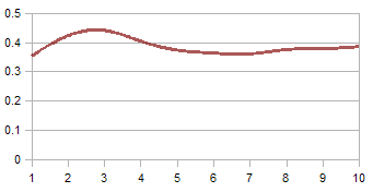
The chart here (right) shows that the Kalman Filter algorithm converges to the true voltage value. Here, I displayed the first 10 iterations and we clearly see the signs of convergence. In 50 or so iterations, it'll converge even better.
To enable the convergence in fewer steps, you should
- Model the system more elegantly
- Estimate the noise more precisely
OK. We're done. The only thing to do is collecting the
 values we've calculated. That's it!
Convergence over iterations
The Kalman Filter algorithm converges to the truth over a few iterations
References
[1] Greg Welch, Gary Bishop, "An Introduction to the Kalman Filter", University of North Carolina at Chapel Hill Department of Computer Science, 2001
[2] M.S.Grewal, A.P. Andrews, "Kalman Filtering - Theory and Practice Using MATLAB", Wiley, 2001


 Rudolf Kalman was born in Budapest, Hungary, and obtained his bachelor's degree in 1953 and
master's degree in 1954 from MIT in electrical engineering. His doctorate in 1957 was from Columbia University.
 Can I deploy Kalman Filter to all Digital Signal Processing problems?
 I've seen lots of papers that use Kalman Filter for a variety of problems, such as noise filtering, sub-space
signal analysis, feature extraction and so on. The bottom line is, you can use Kalman Filter
with a quite approximation and clever modeling.


